Example

Example using default bayesian method on example file

This example data is a subset of the dataset from @Labouyrie2023-yc.

First, the genome sizes are predicted from the taxa:

  results = estimate_genome_size(example_input_file, sep='\t', match_column='TAXID', output_format='input', ci_threshold = 0.3)
  
  #############################################################################
  # Genome size estimation summary:
  #
  #  22.22222 % estimations achieving required precision
  #
       Min.   1st Qu.    Median      Mean   3rd Qu.      Max. 
    3007721   5408472  16980834  23969767  41811396 143278734 
  
  # Estimation status:
  Confidence interval to estimated size ratio > ci_threshold                                                         OK 
                                                         140                                                         40 

Plot genome size histogram per sample

Then, the results can be visualized using the plotting functions provided. This histogram shows the estimated genome sizes for each sample.

  plotted_df = plot_genome_size_histogram(results)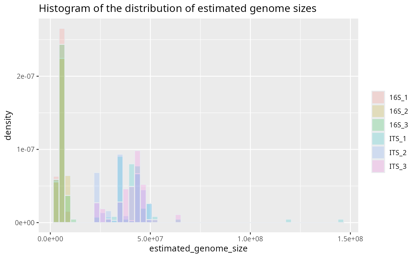

Plot genome size histogram for one sample

  plotted_df = plot_genome_size_histogram(results, only_sample='16S_1')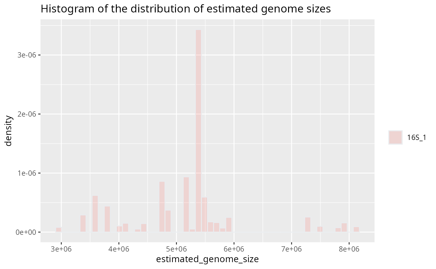

Plot genome size boxplot per sample

This boxplot shows the estimated genome sizes for each sample:

  plotted_df = plot_genome_size_boxplot(results)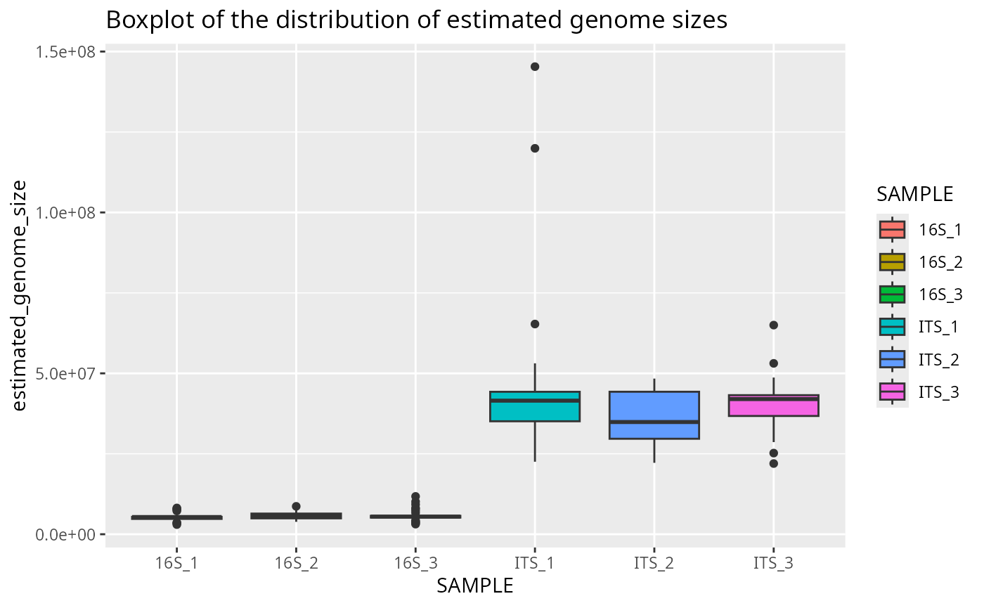

Plot genome size boxplot for one sample

  plotted_df = plot_genome_size_boxplot(results, only_sample='ITS_1')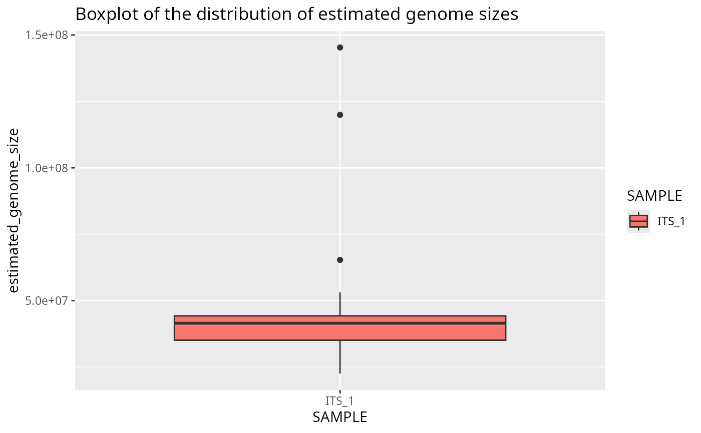

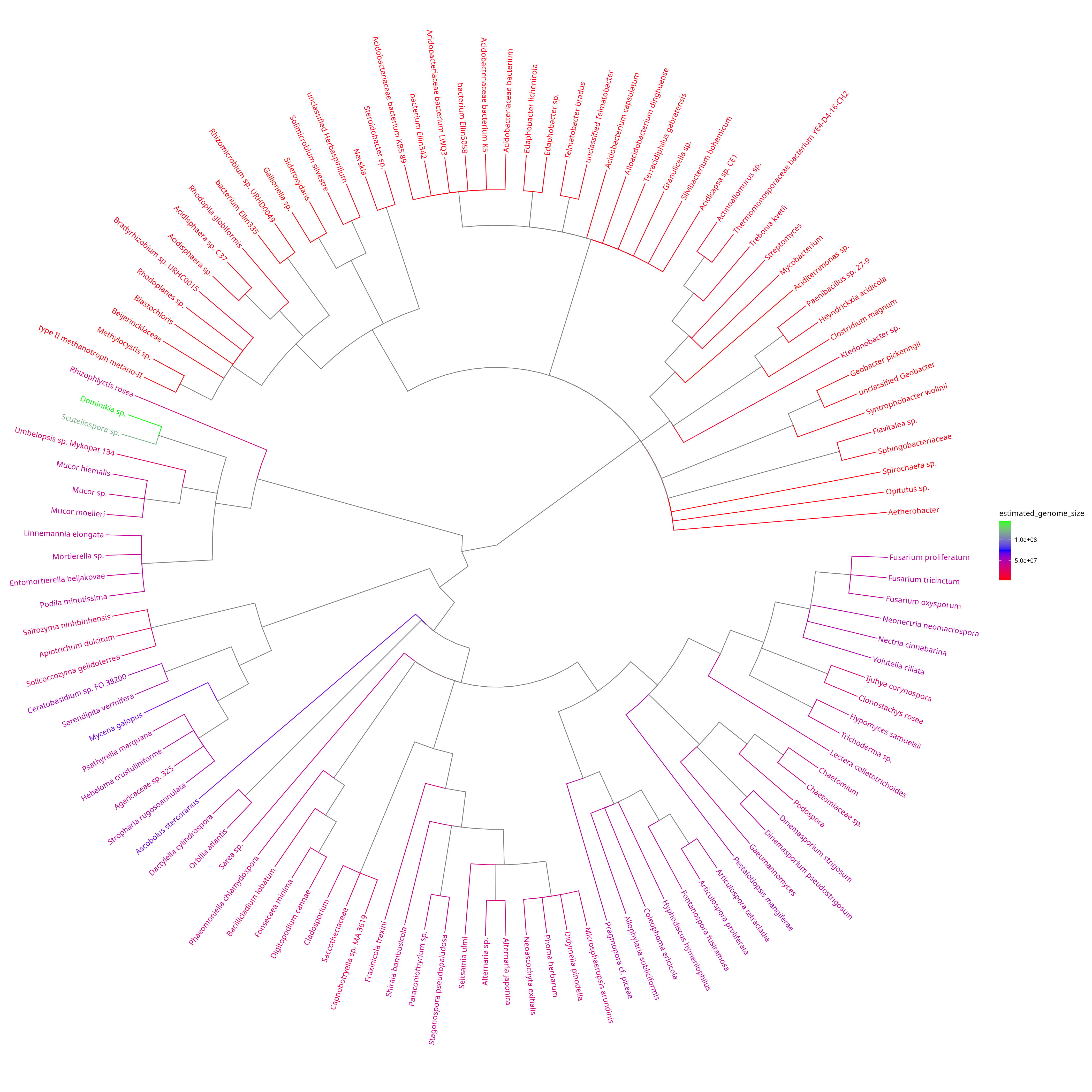
Plot simplified taxonomic tree with colour-coded estimated genome sizes

This tree shows the taxonomic relationships as well as the estimated genome sizes. The difference between the genome size distribution of bacteria (16S marker) and fungi (ITS marker) is visible.

  plotted_df = plot_genome_size_tree(results, refdata_archive_path)

## Untarring reference data
## Using reference data in: /tmp/RtmpzO6rdM/refdata
## Untarring taxonomy
## Using taxonomy: /tmp/RtmpzO6rdM/taxdump